BA Analytics report
Customer Satisfaction Data Analysis in US Airline Services
Table of contents
Abstract
- Motivation
- Data explanation
- Analysis 3.1. Data exploration 3.1.1 Correlation coefficient 3.1.2. Simple linear regression 3.2. Data visualization 3.2.1. Non-Likert-scale factors on satisfaction 3.2.2. Likert-scale factors on satisfaction 3.3. Classification modelling 3.3.1. Tree model / RP, CI tree and Random forest models 3.3.2 Logistic regression model
- Conclusion (omitted) 4.1. Algorithm recommendations (omitted) 4.2. Practical conclusion (omitted) *References
Abstract
With the development of the aviation industry in recent years, there has been surging needs for business analysis about customer convenience in flights, especially in the US. But the bottom line is within a year after this high reputation, in the crisis of this worldwide COVID-19 outbreak, all the airline services and the whole industry got a huge damage on their own businesses due to every country’s current travel restrictions and social distancing policies. So, what we have decided is to analyze how we can suggest to make airlines perform in a quite competitive manner. How will they fly again to risk this situation and attract their customers who want their needs to be satisfied? We analyzed the US airlines customer satisfaction dataset in several ways, following EDA, visualizations with ggplot(), and classification modelling to get more sense of satisfaction analysis. We want to help make breakthroughs now of crisis for airlines by harnessing the analysis skills we’ve learned from this class.
1. Motivation
With the development of the aviation industry in recent years, there has been surging needs for business analysis about customer convenience in flights, especially in the US. According to an article called “Consumer satisfaction in the skies soars to record high in annual airline travel survey” published in CNBC last year, “2019 North American Airline Satisfaction Survey shows travelers gave the industry a record-high score, with the biggest improvements coming from so-called legacy carriers.” It is strongly sure that this improvement about proficiency in customer service has helped airlines record high sales. But the bottom line is within a year after this high reputation, in the crisis of this worldwide COVID-19 outbreak, all the airline services and the whole industry got a huge damage on their own businesses due to every country’s current travel restrictions and social distancing policies. As a matter of fact, “Warren Buffett said Berkshire Hathaway sold its entire stakes in the four largest U.S. carriers as coronavirus devastates travel demand.” last month. The four, which are well-known as four major airlines in US flight industries, “American”, “Delta”, “United”, “Southwest”, “had posted their first quarterly losses in years, and warned of a slow recovery in demand from pre-pandemic levels. Even the CEO of Delta airlines said it could take 2 to 3 years from now.” And not surprisingly, carriers in South Korea suffer the similar situation in industry and businesses. So, what we have decided is to analyze how we can suggest to make airlines perform in a quite competitive manner. How will they fly again to risk this situation and attract their customers who want their needs to be satisfied? And moreover, how can this strategy be coordinated with the country’s travel restrictions and social distancing? We wanted to help make breakthroughs now of crisis for airlines by harnessing the analysis skills we’ve learned from this class.
2. Data Explanation
Our dataset for analysis on the research paper is posted in Kaggle, this dataset deals with US airlines satisfaction survey, and contains 24 columns in about 130000 observations. Short descriptions about 24 columns provided by the publisher of this dataset in Kaggle, are as follows in the table.
sf = read_xlsx("satisfaction.xlsx")
sf
## # A tibble: 129,880 x 24
## id satisfaction_v2 Gender `Customer Type` Age `Type of Travel` Class
## <dbl> <chr> <chr> <chr> <dbl> <chr> <chr>
## 1 11112 satisfied Female Loyal Customer 65 Personal Travel Eco
## 2 110278 satisfied Male Loyal Customer 47 Personal Travel Busi~
## 3 103199 satisfied Female Loyal Customer 15 Personal Travel Eco
## 4 47462 satisfied Female Loyal Customer 60 Personal Travel Eco
## 5 120011 satisfied Female Loyal Customer 70 Personal Travel Eco
## 6 100744 satisfied Male Loyal Customer 30 Personal Travel Eco
## 7 32838 satisfied Female Loyal Customer 66 Personal Travel Eco
## 8 32864 satisfied Male Loyal Customer 10 Personal Travel Eco
## 9 53786 satisfied Female Loyal Customer 56 Personal Travel Busi~
## 10 7243 satisfied Male Loyal Customer 22 Personal Travel Eco
## # ... with 129,870 more rows, and 17 more variables: `Flight Distance` <dbl>,
## # `Seat comfort` <dbl>, `Departure/Arrival time convenient` <dbl>, `Food and
## # drink` <dbl>, `Gate location` <dbl>, `Inflight wifi service` <dbl>,
## # `Inflight entertainment` <dbl>, `Online support` <dbl>, `Ease of Online
## # booking` <dbl>, `On-board service` <dbl>, `Leg room service` <dbl>,
## # `Baggage handling` <dbl>, `Checkin service` <dbl>, Cleanliness <dbl>,
## # `Online boarding` <dbl>, `Departure Delay in Minutes` <dbl>, `Arrival Delay
## # in Minutes` <dbl>As suggested, out of 24 variables, 4 are continuous, 5 are nominal, and 14 are ordinal variables. And we should notice that these ordinal variables include 0, which means NA value out of scale of 1-5, to make sense of preprocessing NA values further. Basically, there has demographic information such as ‘Age’ and ‘Gender’. Moreover, customer type, class (of seats) and flight distance are noted, and additive information about flight delay is also suggested. Most importantly, ‘satisfaction_v2’ summarizes the overall satisfaction by customers who answered this questionnaire. We can guess that there might be correlation between this comprehensive variable and the other service evaluations variables.
3. Data Analysis
3.1. Data exploration
Let’s get down to summarizing our dataset with skimr::skim() function, which has a better performance than summary() function does.
skimr::skim(sf)| Name | sf |
| Number of rows | 129880 |
| Number of columns | 24 |
| _______________________ | |
| Column type frequency: | |
| character | 5 |
| numeric | 19 |
| ________________________ | |
| Group variables | None |
Variable type: character
| skim_variable | n_missing | complete_rate | min | max | empty | n_unique | whitespace |
|---|---|---|---|---|---|---|---|
| satisfaction_v2 | 0 | 1 | 9 | 23 | 0 | 2 | 0 |
| Gender | 0 | 1 | 4 | 6 | 0 | 2 | 0 |
| Customer Type | 0 | 1 | 14 | 17 | 0 | 2 | 0 |
| Type of Travel | 0 | 1 | 15 | 15 | 0 | 2 | 0 |
| Class | 0 | 1 | 3 | 8 | 0 | 3 | 0 |
Variable type: numeric
| skim_variable | n_missing | complete_rate | mean | sd | p0 | p25 | p50 | p75 | p100 | hist |
|---|---|---|---|---|---|---|---|---|---|---|
| id | 0 | 1 | 64940.50 | 37493.27 | 1 | 32470.75 | 64940.5 | 97410.25 | 129880 | ▇▇▇▇▇ |
| Age | 0 | 1 | 39.43 | 15.12 | 7 | 27.00 | 40.0 | 51.00 | 85 | ▃▇▇▅▁ |
| Flight Distance | 0 | 1 | 1981.41 | 1027.12 | 50 | 1359.00 | 1925.0 | 2544.00 | 6951 | ▃▇▂▁▁ |
| Seat comfort | 0 | 1 | 2.84 | 1.39 | 0 | 2.00 | 3.0 | 4.00 | 5 | ▇▇▇▇▅ |
| Departure/Arrival time convenient | 0 | 1 | 2.99 | 1.53 | 0 | 2.00 | 3.0 | 4.00 | 5 | ▇▆▆▇▇ |
| Food and drink | 0 | 1 | 2.85 | 1.44 | 0 | 2.00 | 3.0 | 4.00 | 5 | ▇▇▇▇▆ |
| Gate location | 0 | 1 | 2.99 | 1.31 | 0 | 2.00 | 3.0 | 4.00 | 5 | ▆▆▇▇▅ |
| Inflight wifi service | 0 | 1 | 3.25 | 1.32 | 0 | 2.00 | 3.0 | 4.00 | 5 | ▃▇▇▇▇ |
| Inflight entertainment | 0 | 1 | 3.38 | 1.35 | 0 | 2.00 | 4.0 | 4.00 | 5 | ▃▃▅▇▆ |
| Online support | 0 | 1 | 3.52 | 1.31 | 0 | 3.00 | 4.0 | 5.00 | 5 | ▃▃▅▇▇ |
| Ease of Online booking | 0 | 1 | 3.47 | 1.31 | 0 | 2.00 | 4.0 | 5.00 | 5 | ▃▃▅▇▇ |
| On-board service | 0 | 1 | 3.47 | 1.27 | 0 | 3.00 | 4.0 | 4.00 | 5 | ▂▃▅▇▆ |
| Leg room service | 0 | 1 | 3.49 | 1.29 | 0 | 2.00 | 4.0 | 5.00 | 5 | ▂▅▅▇▇ |
| Baggage handling | 0 | 1 | 3.70 | 1.16 | 1 | 3.00 | 4.0 | 5.00 | 5 | ▁▂▅▇▆ |
| Checkin service | 0 | 1 | 3.34 | 1.26 | 0 | 3.00 | 3.0 | 4.00 | 5 | ▃▃▇▇▆ |
| Cleanliness | 0 | 1 | 3.71 | 1.15 | 0 | 3.00 | 4.0 | 5.00 | 5 | ▁▂▃▇▆ |
| Online boarding | 0 | 1 | 3.35 | 1.30 | 0 | 2.00 | 4.0 | 4.00 | 5 | ▃▅▇▇▇ |
| Departure Delay in Minutes | 0 | 1 | 14.71 | 38.07 | 0 | 0.00 | 0.0 | 12.00 | 1592 | ▇▁▁▁▁ |
| Arrival Delay in Minutes | 393 | 1 | 15.09 | 38.47 | 0 | 0.00 | 0.0 | 13.00 | 1584 | ▇▁▁▁▁ |
In this skim result, this dataset has similar shapes with normal distribution in ages and flight distances. Moreover, many of the respective satisfaction items have 3-4 in mean values, which implies that customers in general are satisfied with airline services overall. Because 5 Likert-scale variables do not count zero as applicable, there are no NA values instead, except for ‘Departure/Arrival delay in minutes’ concerned with special events like delay.
3.1.1. Correlation coefficient
It is better to remain 0 values in 5 Likert-scale variables, rather than changing them with NA. It is because we cannot run correlation tests with numeric variables which have NA values. So, we didn’t consider preprocessing them. The coefficient tables with Pearson correlation tests are as follows.
sf.num = sf %>% mutate(Satisfied_num = ifelse(satisfaction_v2 == 'satisfied', 1, 0), Class_num = case_when(Class == 'Eco' ~ 0, Class == 'Eco Plus' ~ 1, Class == 'Business' ~ 2), Type_num = case_when(`Type of Travel` == 'Personal Travel' ~ 0, `Type of Travel` == 'Business travel' ~ 1), Loyal_num = ifelse(`Customer Type` == 'Loyal Customer', 1, 0))
sf.num = sf.num[, sapply(sf.num, is.numeric)]

corrplot::corrplot(cor(sf.num), method = "shade")
To make correlation tests possible, we had to make variables countable, that is, numeric. Shortly, we converted character variables such as ‘satisfaction_v2’, ‘Type of Travel’, ‘Customer Type’ and ‘Class’ into numeric which are counted on our own. This plot is supposed to be made to get a better understanding regarding the relationship between variables, allowing us to make numeric labels on our own. We counted ‘Eco’ seats, ‘Personal Travel’, ‘disloyal customers’, and ‘neutral or dissatisfied’ with 0, and 1 or 2 with vice versa. Through correlation plot, there seems to be some positive relationship from ‘Seat comfort’ to ‘Gate location’, and from ‘Inflight wifi service’ to ‘Online boarding’. Besides, there seems positive correlation between converted variables. On top of that, regarding ‘Satisfied_num’ which stands for the most comprehensive variable, many of 5 Likert-scale variables seem to have some positive correlations with this variable. So, we can closely look into these parts further.
3.1.2. Simple linear regression
With a simple linear regression test with lm() and tidy(), which summarizes the test in tibble, the result is as follows. The dependent variable is a dummy value labelled ‘Satisfied_num’, which counts 1 with ‘satisfied’ response, and 0 with ‘neutral or dissatisfied’ response.
lm(Satisfied_num~., data = sf.num[,c(2:17, 20)]) %>% broom::tidy()## # A tibble: 17 x 5
## term estimate std.error statistic p.value
## <chr> <dbl> <dbl> <dbl> <dbl>
## 1 (Intercept) -0.675 7.07e-3 -95.5 0.
## 2 Age 0.00104 7.42e-5 14.1 6.79e- 45
## 3 `Flight Distance` -0.00000238 1.07e-6 -2.22 2.62e- 2
## 4 `Seat comfort` 0.0293 1.18e-3 24.9 1.51e-136
## 5 `Departure/Arrival time convenient` -0.0274 9.00e-4 -30.4 1.90e-202
## 6 `Food and drink` -0.0284 1.21e-3 -23.4 2.07e-120
## 7 `Gate location` 0.0191 1.06e-3 18.0 2.51e- 72
## 8 `Inflight wifi service` -0.0152 1.15e-3 -13.3 4.68e- 40
## 9 `Inflight entertainment` 0.141 1.05e-3 134. 0.
## 10 `Online support` 0.0279 1.24e-3 22.5 1.78e-111
## 11 `Ease of Online booking` 0.0559 1.58e-3 35.4 9.54e-274
## 12 `On-board service` 0.0503 1.12e-3 45.1 0.
## 13 `Leg room service` 0.0380 9.68e-4 39.3 0.
## 14 `Baggage handling` 0.00552 1.27e-3 4.34 1.44e- 5
## 15 `Checkin service` 0.0377 9.27e-4 40.7 0.
## 16 Cleanliness 0.00275 1.31e-3 2.09 3.65e- 2
## 17 `Online boarding` 0.00724 1.34e-3 5.40 6.76e- 8boxplot(Age~satisfaction_v2, data = sf, col = "sky blue", border= "purple")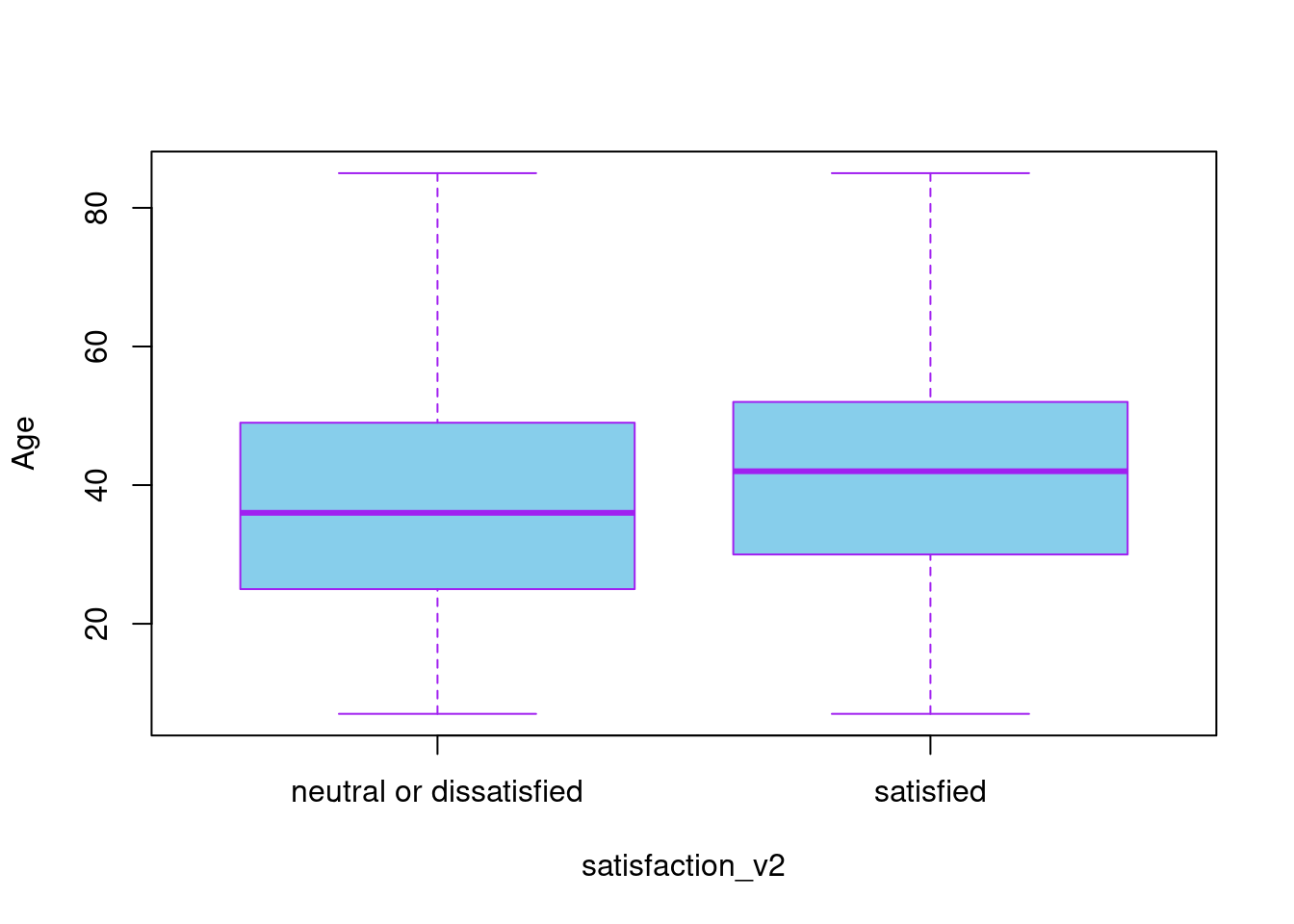
boxplot(sf$`Inflight wifi service`~sf$satisfaction_v2, data = sf, col = "sky blue", border= "purple")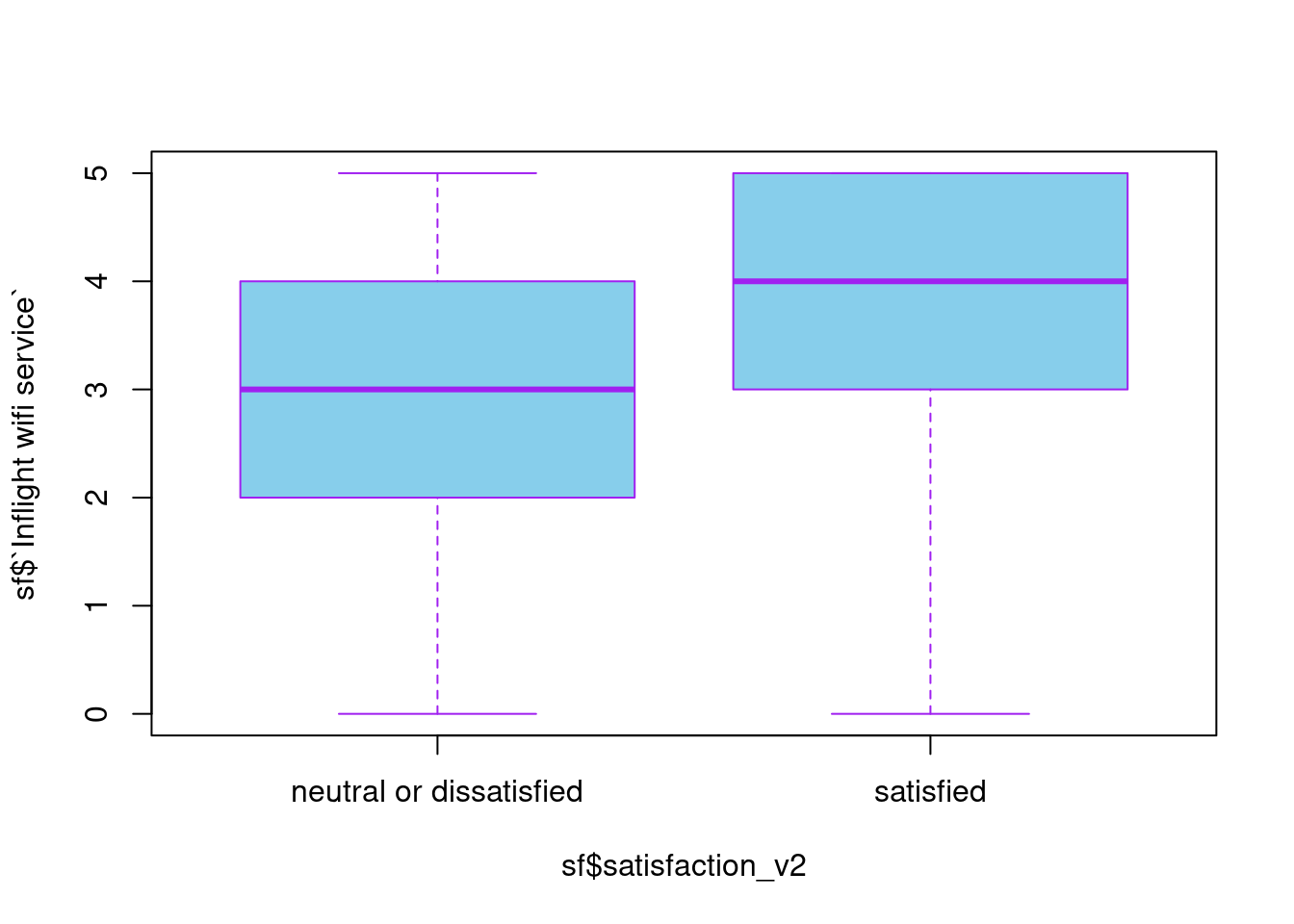
With this simple test, we confirmed significance between overall satisfaction and respective items for airline services. However, we cannot assert a simple linear relationship between them with ease. That is, though we might find them relatable in some senses due to lots of accountable variables in models, we should note that the positive/negative relationships suggested above are not necessarily true. For instance, in the simple lm() model, it is suggested that Age has a negative influence on ‘Satisfied_num’, and even satisfaction on ‘Inflight wifi service’ does too. However, in the boxplots, we may notice more increase both for two numeric variables in satisfied groups than in neutral/dissatisfied groups. Therefore, it would be only enough to conclude that there is an overall positive statistical significance in respective satisfaction items on ‘Satisfied_num’, and a slightly negative significance in ‘Personal travel’, ‘Economy class’, ‘long-distance journey’ groups.
3.2. Data visualization
With EDA above, we found some interesting insights on this dataset. Now we want to articulate these tendencies into ggplot graphs with sophisticated visualizations. What we want here is to make clear which factors ‘satisfaction _v2’, key value in this dataset which stands for customer satisfaction, has much to do with. Here are checklists we would like to confirm, based on some interesting insights suggested above in the last part.
3.2.1. Non-likert scale factors on satisfaction
We already saw that ‘Type of Travel’, ‘Flight distances’ and ‘Customer Type’ has to do with overall satisfaction variables. Therefore, we may look closely at these relationships with geom_bar() and geom_histogram().
(a) Type of travel/Customer type on satisfaction
sf %>%
  ggplot(aes(x = `Type of Travel`, fill = satisfaction_v2)) +
  geom_bar(aes(x = `Type of Travel`))+
  theme_bw()+
  theme(axis.title.x = element_text(size = 15),
        axis.text = element_text(size = 15),
        legend.title = element_text(size = 14),
        legend.text = element_text(size = 13))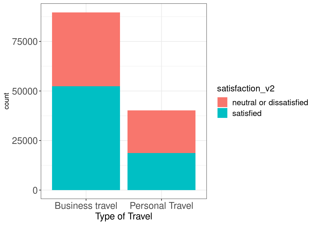
As you see above, Business travelers have satisfied more than personal travels have, and we can easily see the proportional differences in color between two groups.
sf %>%
  ggplot(aes(fill = satisfaction_v2)) +
  geom_bar(aes(x = `Customer Type`)) +
  theme_bw() +
  theme(axis.title.x = element_text(size = 15),
        axis.text = element_text(size = 15),
        legend.title = element_text(size = 14),
        legend.text = element_text(size = 13))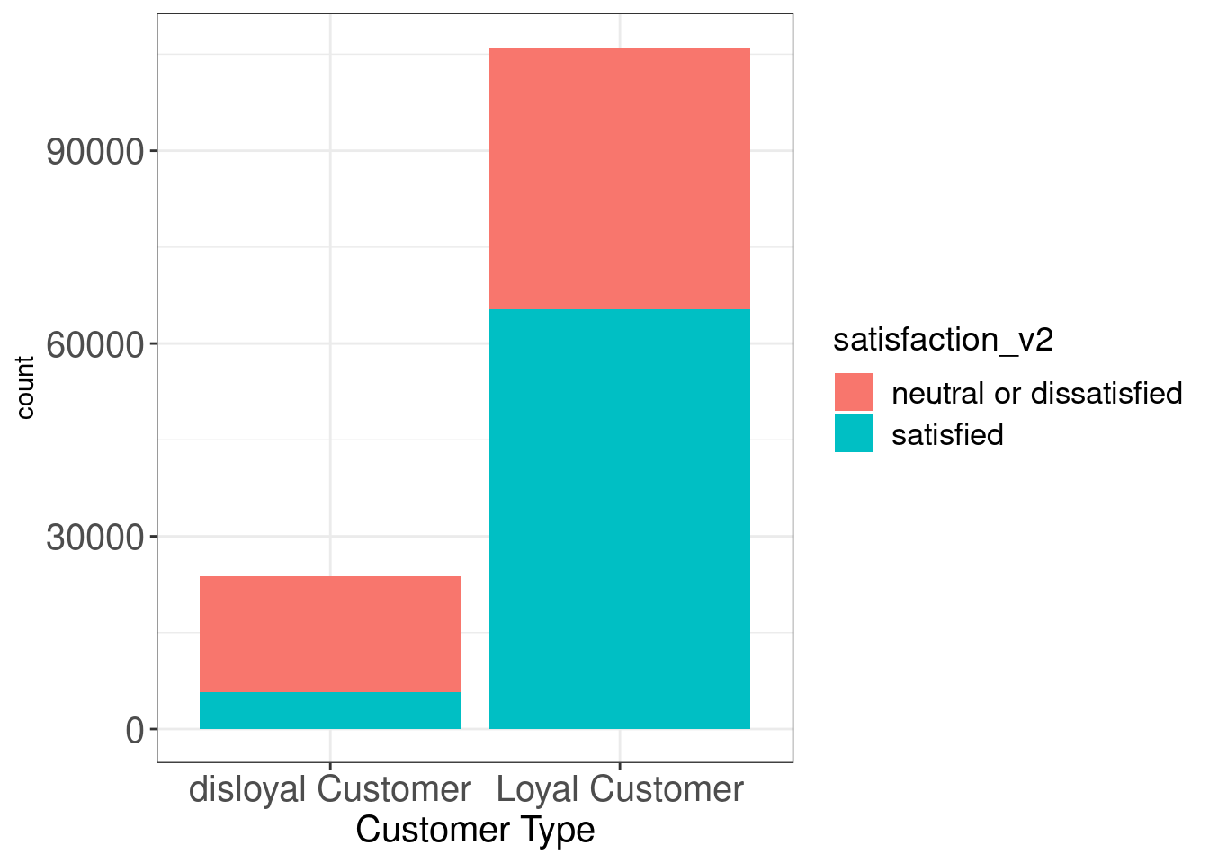
In this graph, although we notice that there are much more loyal customers counted, it is reported that loyal customers tend to be much more satisfied with overall services than their counterparts.
(b) Flight distances on satisfaction
sf %>%
  ggplot(aes(x = `Flight Distance`, fill = satisfaction_v2)) +
  geom_histogram() +
  theme_bw()+
  theme(axis.title.x = element_text(size = 15),
        axis.text = element_text(size = 15),
        legend.title = element_text(size = 14),
        legend.text = element_text(size = 13))
## `stat_bin()` using `bins = 30`. Pick better value with `binwidth`.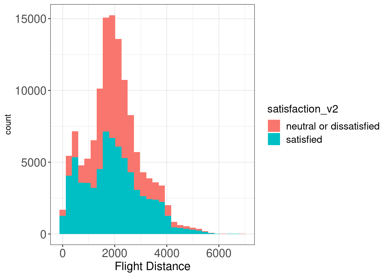
In this histogram suggesting counts on continuous flight distances, we find that only from 1000 to 3000km long, where most customers are covered, satisfaction level is similar with each other while customers are likely to report satisfaction in other ranges. Therefore, it is hard to simply suggest a linear relationship between flight distances and overall satisfaction.
3.2.2. Likert-scale factors on satisfaction
We will focus on two Likert-scale factors, which were reported to have a negative relationship with overall satisfaction. It does not make sense to general thinking, and after looking at the graph we made, we will decide if it is better to get rid of these variables out of model.
sf %>%
  ggplot(aes(x = `Food and drink`, fill = satisfaction_v2)) +
  geom_histogram() +
  theme_bw()+
  theme(axis.title.x = element_text(size = 15),
        axis.text = element_text(size = 15),
        legend.title = element_text(size = 14),
        legend.text = element_text(size = 13))
## `stat_bin()` using `bins = 30`. Pick better value with `binwidth`.
The first one is ‘Food and drink’ satisfaction item. There is a slight increase in proportion of ‘satisfied’ customers in 4-5 point. However, we couldn’t see a clear estimate in EDA, due to 1-3 points where there is no increase in proportion of ‘satisfied’ customers. We can guess as ‘food and drink’ is available at such level, people don’t much care about this item. But since this variable doesn’t seem to harm classification modelling, we can keep that in later models.
sf %>%
  ggplot(aes(x = `Departure/Arrival time convenient`, fill = satisfaction_v2)) +
  geom_histogram() +
  theme_bw()+
  theme(axis.title.x = element_text(size = 15),
        axis.text = element_text(size = 15),
        legend.title = element_text(size = 14),
        legend.text = element_text(size = 13))
## `stat_bin()` using `bins = 30`. Pick better value with `binwidth`.
The second one is ‘Departure/Arrival time convenient’ variable. There shows a similar tendency as ‘Food and drink’. It means that, if they are not so bothered with inconvenience of unpunctuality, they don’t find this variable as important for their satisfaction. However, there is a slight and positive tendency as we see on the graph, which might help classify ‘satisfied’ customers in later models. So, we can keep these two Likert-scale variables.
3.3. Classification modelling
We’ve run classification models which we’ve learned in this course and thought to be proper in this dataset, giving random index with set.seeds(1234) to split train set/test set with probability of 0.7/0.3. And first, here is a simple summary table with sensitivity/specificity and accuracy estimates on each model.
RP Tree Accuracy: 0.8649 Sensitivity/Specificity : 0.8584/0.8703 CI Tree Accuracy: 0.9399 Sensitivity/Specificity : 0.9393/0.9404 Random forest Accuracy: 0.9564 Sensitivity/Specificity : 0.9608/0.9527 Logistic regression Accuracy: 0.8339 Sensitivity/Specificity : (best cut-off; 0.610/ 0.8/0.88) 0.8496/0.8151 Naïve Bayes Accuracy : 0.8103 Sensitivity/Specificity :0.7728/0.8416 * * *
With these 5 models above, ‘Random forest’ classification model showed the best proficiency in accuracy in this case, while Naive Bayes showed the least. All these variables in the model are correlated, not independent each other as presumed in Naive Bayes theory. Now let’s look at the short analysis in each model, except for Naive Bayes model which showed the least proficiency to predict proper satisfaction.
3.3.1. Tree model / RP, CI tree and Random forest models
##########
# RP tree
##########

set.seed(1234) # I checked for 3 seeds, '1234', '1000', '4321'
index = sample(2, nrow(sf), replace = TRUE, prob = c(0.7, 0.3))
trainset = sf[index==1,]
testset = sf[index==2,]
dim(trainset)
## [1] 90994 24dim(testset)## [1] 38886 24sf.rp = rpart::rpart(satisfaction_v2~., data = trainset)
sf.rp## n= 90994
##
## node), split, n, loss, yval, (yprob)
## * denotes terminal node
##
## 1) root 90994 41097 satisfied (0.451645163 0.548354837)
## 2) Inflight entertainment< 3.5 40684 8808 neutral or dissatisfied (0.783502114 0.216497886)
## 4) Seat comfort< 3.5 35562 5178 neutral or dissatisfied (0.854395141 0.145604859)
## 8) Seat comfort>=0.5 33707 3331 neutral or dissatisfied (0.901177797 0.098822203) *
## 9) Seat comfort< 0.5 1855 8 satisfied (0.004312668 0.995687332) *
## 5) Seat comfort>=3.5 5122 1492 satisfied (0.291292464 0.708707536) *
## 3) Inflight entertainment>=3.5 50310 9221 satisfied (0.183283641 0.816716359)
## 6) Ease of Online booking< 3.5 13801 5674 satisfied (0.411129628 0.588870372)
## 12) Inflight entertainment< 4.5 9381 4294 neutral or dissatisfied (0.542266283 0.457733717)
## 24) Online support< 4.5 8110 3222 neutral or dissatisfied (0.602712700 0.397287300) *
## 25) Online support>=4.5 1271 199 satisfied (0.156569630 0.843430370) *
## 13) Inflight entertainment>=4.5 4420 587 satisfied (0.132805430 0.867194570) *
## 7) Ease of Online booking>=3.5 36509 3547 satisfied (0.097154126 0.902845874) *plot(sf.rp, uniform=TRUE, branch=0.1, margin=0.1)
text(sf.rp, all=TRUE, use.n=TRUE)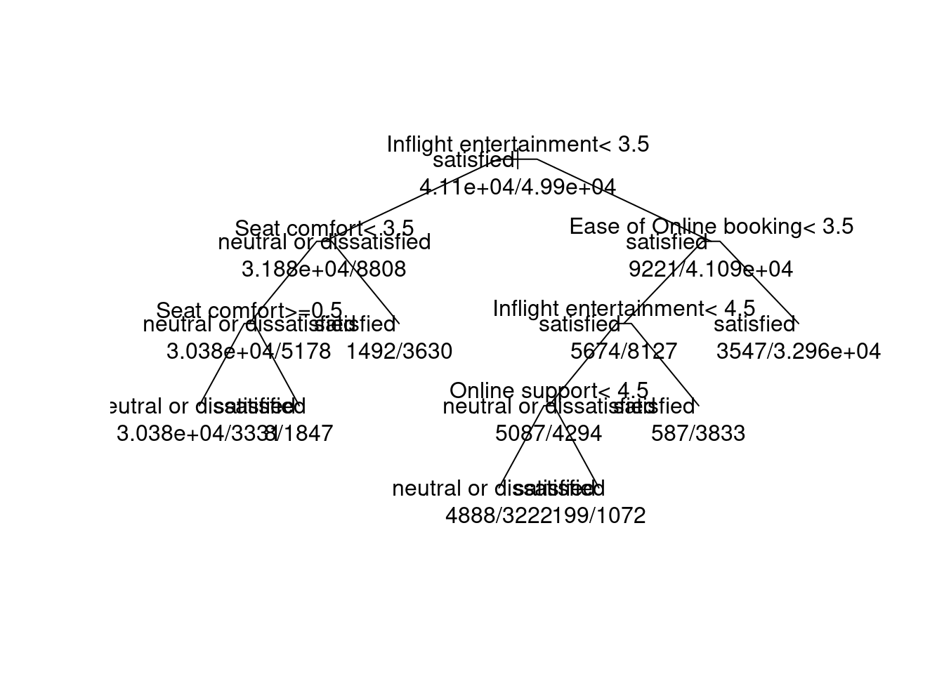
As the plot above in RP tree model suggests, the survey factor which mainly classifies the overall satisfaction was ‘Inflight entertainment’, which we saw the highest coefficient estimate in simple linear regression model. Additionally, we found that there are 5-6 Likert-scale factors mainly included in decision tree.
predictions = predict(sf.rp, testset, type="class")
table(predictions, testset$satisfaction_v2)
##
## predictions neutral or dissatisfied satisfied
## neutral or dissatisfied 15191 2749
## satisfied 2505 18441confusionMatrix(table(predictions, testset$satisfaction_v2))## Confusion Matrix and Statistics
##
##
## predictions               neutral or dissatisfied satisfied
##   neutral or dissatisfied                   15191      2749
##   satisfied                                  2505     18441
##
## Accuracy : 0.8649
## 95% CI : (0.8614, 0.8683)
## No Information Rate : 0.5449
## P-Value [Acc > NIR] : < 2.2e-16
##
## Kappa : 0.7279
##
## Mcnemar's Test P-Value : 0.000801
##
## Sensitivity : 0.8584
## Specificity : 0.8703
## Pos Pred Value : 0.8468
## Neg Pred Value : 0.8804
## Prevalence : 0.4551
## Detection Rate : 0.3907
## Detection Prevalence : 0.4613
## Balanced Accuracy : 0.8644
##
## 'Positive' Class : neutral or dissatisfied
## rpart::plotcp(sf.rp)
This is the result graph on plotcp(). We saw that this RP tree showed the least X-Error on Y axis, when separated with 7 groups. That’s why there are only 6 main variables in our RP tree model. However, we can go further with CI tree model after converting some character variables into factor variables to apply this model. As suggested above the table, CI tree show high accuracy over .9 and well-balanced sensitivity/specificity for each, without any further pruning process since this method uses significance to prune the tree.
##########
# CI tree
##########

# Pre-processing before prdictions

sf$satisfaction_v2 = as.factor(sf$satisfaction_v2)
sf$Gender= as.factor(sf$Gender)
sf$`Customer Type` = as.factor(sf$`Customer Type`)
sf$`Type of Travel` = as.factor(sf$`Type of Travel`)
sf$Class = as.factor(sf$Class)

sf.name = sf %>% colnames() %>% str_replace_all(" ","")
sf.df.name = sf %>% setNames(sf.name)

trainset.ci = sf[index==1,]
testset.ci = sf[index==2,]

sf.ci = ctree(satisfaction_v2 ~ ., data=trainset.ci)
# sf.ci
# plot(sf.ci)

predictions = predict(sf.ci, testset.ci)
table(predictions, testset.ci$satisfaction_v2)
##
## predictions neutral or dissatisfied satisfied
## neutral or dissatisfied 16621 1263
## satisfied 1075 19927confusionMatrix(table(predictions, testset.ci$satisfaction_v2))## Confusion Matrix and Statistics
##
##
## predictions               neutral or dissatisfied satisfied
##   neutral or dissatisfied                   16621      1263
##   satisfied                                  1075     19927
##
## Accuracy : 0.9399
## 95% CI : (0.9375, 0.9422)
## No Information Rate : 0.5449
## P-Value [Acc > NIR] : < 2e-16
##
## Kappa : 0.8789
##
## Mcnemar's Test P-Value : 0.00011
##
## Sensitivity : 0.9393
## Specificity : 0.9404
## Pos Pred Value : 0.9294
## Neg Pred Value : 0.9488
## Prevalence : 0.4551
## Detection Rate : 0.4274
## Detection Prevalence : 0.4599
## Balanced Accuracy : 0.9398
##
## 'Positive' Class : neutral or dissatisfied
## ##########
# Random Forest
##########
sf = sf[,2:22]
sf.name = sf %>% colnames() %>% str_replace_all(" ","")
sf.df.name = sf %>% setNames(sf.name)
trainset.rf = sf.df.name[index==1,]
testset.rf = sf.df.name[index==2,]
sf.rf = randomForest(satisfaction_v2 ~ Gender+CustomerType+Age+TypeofTravel+Class+FlightDistance+Seatcomfort+Foodanddrink+Gatelocation+Inflightwifiservice+Inflightentertainment+Onlinesupport+EaseofOnlinebooking+Legroomservice+Baggagehandling+Checkinservice+Cleanliness+Onlineboarding, data=trainset.rf, mtry = 4,importance=T)
sf.rf##
## Call:
## randomForest(formula = satisfaction_v2 ~ Gender + CustomerType + Age + TypeofTravel + Class + FlightDistance + Seatcomfort + Foodanddrink + Gatelocation + Inflightwifiservice + Inflightentertainment + Onlinesupport + EaseofOnlinebooking + Legroomservice + Baggagehandling + Checkinservice + Cleanliness + Onlineboarding, data = trainset.rf, mtry = 4, importance = T)
## Type of random forest: classification
## Number of trees: 500
## No. of variables tried at each split: 4
##
## OOB estimate of error rate: 4.39%
## Confusion matrix:
## neutral or dissatisfied satisfied class.error
## neutral or dissatisfied 39466 1631 0.03968660
## satisfied 2365 47532 0.04739764importance(sf.rf)## neutral or dissatisfied satisfied MeanDecreaseAccuracy
## Gender 93.80317 86.07941 114.76980
## CustomerType 90.62215 97.23443 117.30727
## Age 65.84208 53.35518 77.86496
## TypeofTravel 81.97683 62.62632 94.94336
## Class 52.90785 49.97860 57.42750
## FlightDistance 44.82861 54.04602 56.86789
## Seatcomfort 163.62877 70.20255 121.94201
## Foodanddrink 54.37578 54.90897 67.74233
## Gatelocation 64.86997 42.31150 45.43890
## Inflightwifiservice 29.54222 45.56537 42.59609
## Inflightentertainment 86.65404 95.08923 102.27934
## Onlinesupport 98.93648 67.07348 108.63742
## EaseofOnlinebooking 50.41784 64.89189 70.74521
## Legroomservice 58.65977 57.94695 72.16473
## Baggagehandling 87.30701 55.29611 93.06569
## Checkinservice 129.61726 66.43225 138.20110
## Cleanliness 84.03315 43.18748 80.70073
## Onlineboarding 45.57739 50.95123 55.29616
## MeanDecreaseGini
## Gender 1530.6700
## CustomerType 2093.1213
## Age 1649.5433
## TypeofTravel 1414.5922
## Class 1693.8840
## FlightDistance 1927.4891
## Seatcomfort 6118.6172
## Foodanddrink 1903.5499
## Gatelocation 1144.2234
## Inflightwifiservice 832.5739
## Inflightentertainment 9564.7296
## Onlinesupport 3157.4321
## EaseofOnlinebooking 3629.4027
## Legroomservice 2127.8369
## Baggagehandling 1364.9374
## Checkinservice 1286.3479
## Cleanliness 1363.4651
## Onlineboarding 1628.1457predictions = predict(sf.rf, testset.rf)
table(predictions, testset.rf$satisfaction_v2)##
## predictions neutral or dissatisfied satisfied
## neutral or dissatisfied 16998 991
## satisfied 698 20199confusionMatrix(table(predictions, testset.rf$satisfaction_v2))## Confusion Matrix and Statistics
##
##
## predictions               neutral or dissatisfied satisfied
##   neutral or dissatisfied                   16998       991
##   satisfied                                   698     20199
##
## Accuracy : 0.9566
## 95% CI : (0.9545, 0.9586)
## No Information Rate : 0.5449
## P-Value [Acc > NIR] : < 2.2e-16
##
## Kappa : 0.9125
##
## Mcnemar's Test P-Value : 1.203e-12
##
## Sensitivity : 0.9606
## Specificity : 0.9532
## Pos Pred Value : 0.9449
## Neg Pred Value : 0.9666
## Prevalence : 0.4551
## Detection Rate : 0.4371
## Detection Prevalence : 0.4626
## Balanced Accuracy : 0.9569
##
## 'Positive' Class : neutral or dissatisfied
## On top of that, we saw the random forest model, well-known as ensemble learning which harnesses ‘bagging’ to fix the errors in other decision trees, shows the best proficiency in predicting the overall customer satisfaction variable. Moreover, we can sophisticate this model with changing parameters in the randomforest() function, such as ntree and mtry. The only thing concerned with this model is computing time, though this doesn’t make differences in proficiency of this model. We ran for loop to calculate the best parameters in random forest. And with ntree of 500 and mtry of 5, this model showed the highest accuracy of .9572 in prediction.
ntree = c(400, 500, 600)
mtry = c(3:5)
param = data.frame(n = ntree, m = mtry)

for (i in param$n){
  cat('ntree=', i, '\n')
  for (j in param$m){
    cat('mtry')
    model_sf = randomForest(satisfaction_v2~Gender+CustomerType+Age+TypeofTravel+Class+FlightDistance+Seatcomfort+Foodanddrink+Gatelocation+Inflightwifiservice+Inflightentertainment+Onlinesupport+EaseofOnlinebooking+Legroomservice+Baggagehandling+Checkinservice+Cleanliness+Onlineboarding, data=trainset.rf, ntree = i, mtry = j,importance=T)

predictions.1 = predict(model_sf, testset.rf)
table(predictions.1, testset.rf$satisfaction_v2)
confusionMatrix(table(predictions.1, testset.rf$satisfaction_v2))
  }
}
3.2.2. Logistic regression model
##########
# Logistic regrssion
##########

sf.lr = sf %>%
  mutate(satisfaction_v2 = ifelse(satisfaction_v2 == 'satisfied', 1, 0))

trainset.lr = sf.lr[index==1,]
testset.lr = sf.lr[index==2,]

fit = glm(satisfaction_v2 ~ ., data=trainset.lr, family=binomial)
summary(fit)
##
## Call:
## glm(formula = satisfaction_v2 ~ ., family = binomial, data = trainset.lr)
##
## Deviance Residuals:
## Min 1Q Median 3Q Max
## -3.0167 -0.5796 0.1980 0.5245 3.6593
##
## Coefficients:
## Estimate Std. Error z value Pr(>|z|)
## (Intercept) -6.772e+00 7.780e-02 -87.040 < 2e-16 ***
## GenderMale -9.555e-01 1.955e-02 -48.876 < 2e-16 ***
## `Customer Type`Loyal Customer 1.979e+00 2.977e-02 66.470 < 2e-16 ***
## Age -7.613e-03 6.791e-04 -11.210 < 2e-16 ***
## `Type of Travel`Personal Travel -7.821e-01 2.787e-02 -28.060 < 2e-16 ***
## ClassEco -7.290e-01 2.529e-02 -28.829 < 2e-16 ***
## ClassEco Plus -8.156e-01 3.894e-02 -20.946 < 2e-16 ***
## `Flight Distance` -1.365e-04 1.017e-05 -13.426 < 2e-16 ***
## `Seat comfort` 2.960e-01 1.097e-02 26.969 < 2e-16 ***
## `Departure/Arrival time convenient` -2.045e-01 8.084e-03 -25.303 < 2e-16 ***
## `Food and drink` -2.157e-01 1.111e-02 -19.416 < 2e-16 ***
## `Gate location` 1.099e-01 9.097e-03 12.084 < 2e-16 ***
## `Inflight wifi service` -7.535e-02 1.053e-02 -7.157 8.26e-13 ***
## `Inflight entertainment` 6.836e-01 9.856e-03 69.354 < 2e-16 ***
## `Online support` 8.657e-02 1.072e-02 8.078 6.58e-16 ***
## `Ease of Online booking` 2.244e-01 1.381e-02 16.250 < 2e-16 ***
## `On-board service` 3.031e-01 9.840e-03 30.808 < 2e-16 ***
## `Leg room service` 2.167e-01 8.344e-03 25.970 < 2e-16 ***
## `Baggage handling` 9.123e-02 1.108e-02 8.234 < 2e-16 ***
## `Checkin service` 2.955e-01 8.245e-03 35.843 < 2e-16 ***
## Cleanliness 1.045e-01 1.147e-02 9.118 < 2e-16 ***
## `Online boarding` 1.691e-01 1.177e-02 14.368 < 2e-16 ***
## ---
## Signif. codes: 0 '***' 0.001 '**' 0.01 '*' 0.05 '.' 0.1 ' ' 1
##
## (Dispersion parameter for binomial family taken to be 1)
##
## Null deviance: 125292 on 90993 degrees of freedom
## Residual deviance: 70489 on 90972 degrees of freedom
## AIC: 70533
##
## Number of Fisher Scoring iterations: 5pred = predict(fit, testset, type="response")
predictions = (pred <.5)
table(predictions, testset.lr$satisfaction_v2)##
## predictions 0 1
## FALSE 3272 18002
## TRUE 14424 3188testset.lr$manual_l=ifelse(testset.lr$satisfaction_v2==1, FALSE, TRUE)
table(predictions, testset.lr$manual_l)##
## predictions FALSE TRUE
## FALSE 18002 3272
## TRUE 3188 14424confusionMatrix(table(predictions, testset.lr$manual_l))## Confusion Matrix and Statistics
##
##
## predictions FALSE  TRUE
##       FALSE 18002  3272
##       TRUE   3188 14424
##
## Accuracy : 0.8339
## 95% CI : (0.8301, 0.8376)
## No Information Rate : 0.5449
## P-Value [Acc > NIR] : <2e-16
##
## Kappa : 0.6649
##
## Mcnemar's Test P-Value : 0.3018
##
## Sensitivity : 0.8496
## Specificity : 0.8151
## Pos Pred Value : 0.8462
## Neg Pred Value : 0.8190
## Prevalence : 0.5449
## Detection Rate : 0.4629
## Detection Prevalence : 0.5471
## Balanced Accuracy : 0.8323
##
## 'Positive' Class : FALSE
## # find the best cut-off
sf.roc=roc(testset.lr$manual_l, pred)
plot(sf.roc)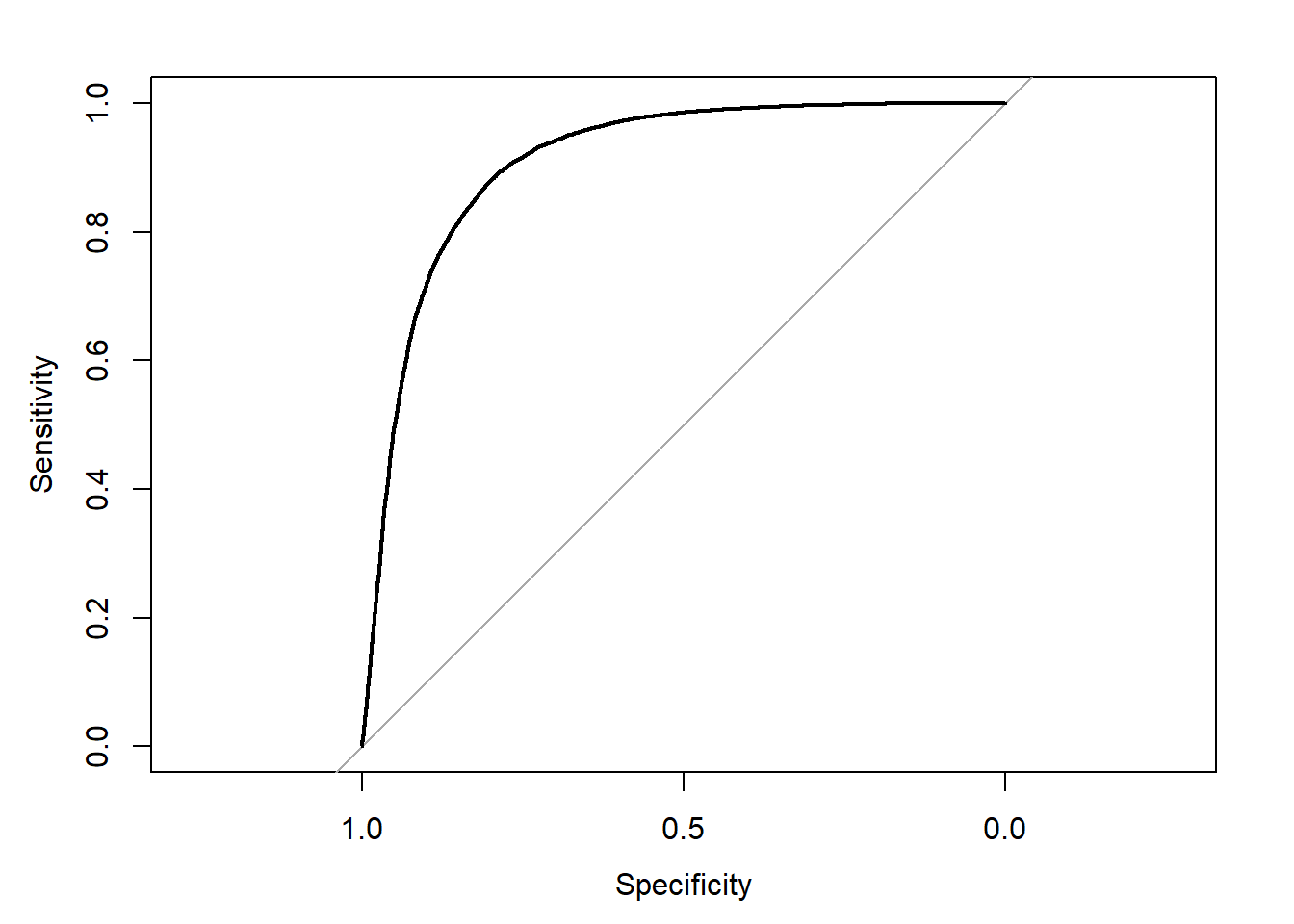
coords(sf.roc, "best")## Warning in coords.roc(sf.roc, "best"): The 'transpose' argument to FALSE
## by default since pROC 1.16. Set transpose = TRUE explicitly to revert to
## the previous behavior, or transpose = TRUE to silence this warning. Type
## help(coords_transpose) for additional information.## threshold specificity sensitivity
## 1 0.6104963 0.800991 0.8798599And, here is the threshold graph for the best cut-off in logistic regression model. We also ran for logistic regression model, which is good to set the best cut-off for sensitivity/specificity. For running, we should pre-process the ‘satisfaction_v2’ with making it as a numeric variable, because this model assumes a binomial family in Y value. The best cut-off in both sensitivity and specificity is 0.610, and the best result is 0.8/0.88 for each. Plus, with that, we should notice these are in fact reversed estimates, because we should assume that the actual positive value is ‘neutral/dissatisfied’, which should be more accurately predicted to improve customer services of US airlines.