SOTU Text Analysis
도입
데이터 호출 및 전처리
UC Santa Barbara의 ‘The American Presidency project’에서는 매해 단위로 수집한 역대 미국 대통령의 의회 국정연설문을 텍스트 데이터로 아카이빙하고 있다. ’State of the Union’(SOTU) 데이터셋이 바로 그것인데, 초대 대통령 조지 워싱턴(1789~1797 재임)부터 45대 대통령 도널드 트럼프(2017~)의 구두/서면 연설문이 txt 파일 형태로 정리되어 있다. URL 역시 크롤링하기 간편한 규칙성을 띠고 있어 txt 파일데이터 전량을 손쉽게 크롤링할 수 있다. URL 링크 접근과 크롤링을 위해 정리된 메타데이터 엑셀 파일과, 정리된 연설문 파일을 불러오는 것부터 시작하자.
library(tidyverse)
library(tidytext)
library(tm)
library(quanteda)list.files()stu = read_csv("STU_address_metadata.csv") %>% as_tibble()##
## ─ Column specification ────────────────────────────
## cols(
## label = col_character(),
## href = col_character(),
## president = col_character(),
## president_no = col_character(),
## years = col_character(),
## title = col_character(),
## date = col_character(),
## doc_id = col_double()
## )head(stu)## # A tibble: 6 x 8
## label href president president_no years title date doc_id
## <chr> <chr> <chr> <chr> <chr> <chr> <chr> <dbl>
## 1 2017 https://www.p… Donald J.… 45th 2017 … Address Bef… Febru… 1
## 2 2018 https://www.p… Donald J.… 45th 2017 … Address Bef… Janua… 2
## 3 2019 https://www.p… Donald J.… 45th 2017 … Address Bef… Febru… 3
## 4 2020 https://www.p… Donald J.… 45th 2017 … Address Bef… Febru… 4
## 5 2013 https://www.p… Barack Ob… 44th 2009 … Address Bef… Febru… 5
## 6 2014 https://www.p… Barack Ob… 44th 2009 … Address Bef… Janua… 6이번 텍스트 데이터 전처리는 tidytext 패키지의 unnest_tokens() 함수를 이용한다. 연설문 텍스트 파일을 tibble 형태로 불러온 후, 연결된 문장을 단어별로 구획해보자.
doc_1 = read_lines("doc_1.txt") %>% as_tibble() %>%
  unnest_tokens(words, value, token="words")

head(doc_1, n = 10)
## # A tibble: 10 x 1
## words
## <chr>
## 1 thank
## 2 you
## 3 very
## 4 much
## 5 mr
## 6 speaker
## 7 mr
## 8 vice
## 9 president
## 10 members평균 단어 수 계산
보기와 같이 띄어쓰기를 기준으로 한 어절 단위로 연설문이 처리되었음을 알 수 있다. 이제 우리는 해당 텍스트 데이터의 기본적인 분석에 착수할 수 있다. 우선 연설문당 평균 단어수를 계산해보자.
tmp = stu %>% as_tibble() %>%
  select(president, doc_id, president_no) %>%
  arrange(doc_id)

wnum = list()
for (i in 1:max(tmp$doc_id)){
  doc_n = read_lines(str_c("doc_", as.character(i),".txt")) %>% as_tibble %>%
    unnest_tokens(words, value, token = "words")
  wnum = bind_rows(wnum, count(doc_n))
}
anyNA(cbind(tmp, wnum))
## [1] FALSEA1 = cbind(tmp, wnum) %>% as_tibble
meanword = list()
mw = list()
pname = list()
tmpname = list()
for (i in 1:42){
mw = mean(A1$n[A1$president == unique(A1$president)[i]])
meanword[[i]] = mw
tmpname = as.character(unique(A1$president)[i])
pname[[i]] = tmpname
}
a = as.data.frame(cbind(meanword, pname))
a = a[nrow(a):1,]이때 22대, 24대 대통령은 ’Grover Cleveland’로, 연속 연임 대통령이 아닌 유일한 2선 대통령이므로 별도의 전처리를 거쳐야 한다.
round(mean(A1$n[A1$president_no == "22nd"]),0) # 22대 대통령 재임시절 Cleveland## [1] 13401round(mean(A1$n[A1$president_no == "24th"]),0) # 24대 대통령 재임시절 Cleveland## [1] 14652a$meanword[21] == as.numeric(a$meanword[a$pname == "Grover Cleveland"])## [1] TRUEb = round(as.numeric(a$meanword[-21])) %>% as_tibble()
c = b[1:19,]
c[20:22, ] = c(13401, 13668, 14652)
c[23:43,] = b[21:41,]인칭대명사 사용 빈도 계산
1~3인칭 단/복수 인칭대명사의 빈도 역시 우리에게 많은 것을 알려줄 수 있다. 대통령별 각 대명사의 사용 빈도를 알아보자. 이때 unnest_token() 함수로 구분된 어절은 모두 소문자로 시작하므로 결측을 배제하기 위한 별도의 전처리가 필요 없다. 대명사 종류별 수집할 어휘는 다음과 같다. (2인칭의 경우 단/복수 형태의 구분이 없으므로 함께 고려한다.)
1인칭 단수 : i, my, me, mine 1인칭 복수 : we, us, our, ours 2인칭 단수/복수 : you, your, yours 3인칭 단수 : he, she, his, her, him 3인칭 복수 : they, their, them, theirs
tmp_2 = tibble()
for (i in 1:max(tmp$doc_id)){
  doc_n = read_lines(str_c("doc_",as.character(i),".txt")) %>% as_tibble %>%
    unnest_tokens(words, value, token = "words")
  tmp_2[i,1] = nrow(doc_n)
  tmp_2[i,2] = sum(length(doc_n$words[doc_n$words == "i"]), length(doc_n$words[doc_n$words == "my"]),
  length(doc_n$words[doc_n$words == "me"]), length(doc_n$words[doc_n$words == "mine"]))
  tmp_2[i,3] = sum(length(doc_n$words[doc_n$words == "we"]), length(doc_n$words[doc_n$words == "our"]),
  length(doc_n$words[doc_n$words == "us"]), length(doc_n$words[doc_n$words == "ours"]))
  tmp_2[i,4] = sum(length(doc_n$words[doc_n$words == "you"]), length(doc_n$words[doc_n$words == "your"]),
  length(doc_n$words[doc_n$words == "yours"]))
  tmp_2[i,5] = sum(length(doc_n$words[doc_n$words == "he"]), length(doc_n$words[doc_n$words == "she"]),
  length(doc_n$words[doc_n$words == "his"]), length(doc_n$words[doc_n$words == "her"]),
  length(doc_n$words[doc_n$words == "him"]))
  tmp_2[i,6] = sum(length(doc_n$words[doc_n$words == "they"]), length(doc_n$words[doc_n$words == "their"]),
  length(doc_n$words[doc_n$words == "them"]), length(doc_n$words[doc_n$words == "theirs"]))
}
A2 = inner_join(A1, tmp_2, c("n"="...1")) %>% unique()

head(A2)
## # A tibble: 6 x 9
## president doc_id president_no n ...2 ...3 ...4 ...5 ...6
## <chr> <dbl> <chr> <int> <int> <int> <int> <int> <int>
## 1 Donald J. Trump 1 45th 5096 54 237 29 29 60
## 2 Donald J. Trump 2 45th 5926 51 253 52 62 80
## 3 Donald J. Trump 3 45th 5798 63 230 47 42 47
## 4 Donald J. Trump 4 45th 6387 81 199 91 65 33
## 5 Barack Obama 5 44th 6897 46 299 22 33 69
## 6 Barack Obama 6 44th 7114 74 235 30 56 71A2_1 = tibble()
A2_1 = A2 %>%
mutate(...2 = 100*...2/n,
...3 = 100*...3/n,
...4 = 100*...4/n,
...5 = 100*...5/n,
...6 = 100*...6/n)
A2_2 = tibble()
for (i in 1:42){
A2_2[i,1] = unique(A2_1$president)[i]
A2_2[i,2] = round(mean(A2_1$n[A2_1$president == unique(A2_1$president)[i]]),0)
A2_2[i,3] = round(mean(A2_1$...2[A2_1$president == unique(A2_1$president)[i]]),2)
A2_2[i,4] = round(mean(A2_1$...3[A2_1$president == unique(A2_1$president)[i]]),2)
A2_2[i,5] = round(mean(A2_1$...4[A2_1$president == unique(A2_1$president)[i]]),2)
A2_2[i,6] = round(mean(A2_1$...5[A2_1$president == unique(A2_1$president)[i]]),2)
A2_2[i,7] = round(mean(A2_1$...6[A2_1$president == unique(A2_1$president)[i]]),2)
}
A2_2[22,] ## Grover Cleveland
A2_2 = A2_2[-22,]A2_2 %>%
mutate(rown = row_number()) %>% arrange(desc(rown)) %>%
rename("president" = ...1, "totalwords" = ...2, "I" = ...3, "we" = ...4, "you" = ...5, "he/she" = ...6, "they" = ...7)## # A tibble: 41 x 8
## president totalwords I we you `he/she` they rown
## <chr> <dbl> <dbl> <dbl> <dbl> <dbl> <dbl> <int>
## 1 George Washington 2082 1.04 1.25 0.83 0.17 1.18 41
## 2 John Adams 1789 0.9 1.81 0.56 0.31 1.16 40
## 3 Thomas Jefferson 2584 0.47 2.4 0.53 0.2 1.77 39
## 4 James Madison 2711 0.34 1.38 0.17 0.51 0.98 38
## 5 James Monroe 5290 0.32 1.25 0.12 0.36 1.19 37
## 6 John Quincy Adams 7774 0.18 1.15 0.1 0.32 1.28 36
## 7 Andrew Jackson 11273 0.84 1.32 0.27 0.37 1.11 35
## 8 Martin van Buren 11365 0.56 0.83 0.23 0.16 1.34 34
## 9 John Tyler 8517 0.570 0.73 0.32 0.45 0.75 33
## 10 James K. Polk 18054 0.39 1.28 0.12 0.84 1.25 32
## # … with 31 more rows시각화
대통령별 평균 단어 수 시각화
우선 처음에 구한 대통령별 연설문 평균 단어 수를 시각화해보자.
A2_3 = tibble()
for (i in 0:42){
  A2_3[i+1,1] = unique(A2_1$president_no)[43-i]
  A2_3[i+1,2] = unique(A2_1$president)[43-i]}
for (i in 1:19){
A2_3[c(i,i+1),2] = A2_3[c(i+1, i),2]}
A2_3[20,2] = unique(A2_1$president)[22]

A3_1 = bind_cols(A2_3, c)
A3_1 = A3_1 %>%
  rename("president_no" = ...1, "president" = ...2)
A3_1 = A3_1 %>%
mutate(president_no = str_extract(president_no,"[[:digit:]]{1,2}"),
president_no = as.numeric(president_no))
A3_1 %>%
ggplot(aes(x = 46-president_no, y = value)) +
geom_point(size = 2) +
geom_line() +
labs(x="President of the United States",
y="Average number of words addressed") +
ylim(c(1000,25000)) +
scale_x_continuous(breaks=46-A3_1$president_no,
labels=A3_1$president) +
theme(axis.text.x.bottom = element_text(angle = 45)) +
theme_light()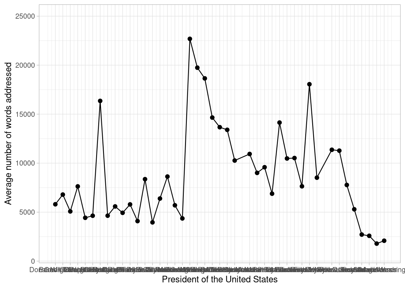
이때, 대통령별 변화량에 주목하기보다 시대 변화에 따른 추이를 보고 싶다면 축을 세로로 돌리면 좀 더 보기 편할 것이다. ggplot 패키지의 coord_flip() 함수를 이용하면 된다. 추가적으로 추세선과 함께 그래프를 보면 전반적인 추이를 검토하기 더욱 편할 것이다. 이때 추세선은 전반적이고 유동적인 추이를 시각화하여 제공하고자 함이 주 사용목적이므로 geom_smooth(method = ‘loess’)를 이용하자.
A3_1 %>%
  ggplot(aes(x = 46-president_no, y = value)) +
  geom_point(size = 2) +
  geom_line() +
  geom_smooth() +
  labs(x="President of the United States",
       y="Average number of words addressed") +
  ylim(c(1000,25000)) +
  scale_x_continuous(breaks=46-A3_1$president_no,
                     labels=A3_1$president) +
  coord_flip() +
  theme_light()
## `geom_smooth()` using method = 'loess' and formula 'y ~ x'
당시 미국의 역사적 흐름과 결부해 위와 같이 평균 단어 수가 변화하는 추세를 분석해보면 다음과 같다. 개국부터 남북전쟁, 독립전쟁 및 노예제 폐지를 지나 20세기 초반의 경제 호황기에 접어들기까지 미국은 정치 부문의 민주적 발전과 경제 부문의 양적 팽창을 도모해 왔다. 이에 따라 대통령은 자신의 국정 연설에 국가가 나아갈 방향에 대한 제언 등 여러 강조 사항을 담고자 했을 것이다. 그런데, 27대 대통령 윌리엄 태프트 재임 기간에서 28대 대통령 우드로 윌슨 재임 기간으로 넘어가는 지점에서는 평균 단어 수의 추이가 급감하는데, 그 이유는 앞서 언급한 역사적 맥락과 비교해 훨씬 명확하다. USCB(Univ. Santa Barbara)의 한 에세이에 따르면, 3대 대통령 토머스 제퍼슨부터 28대 대통령 우드로 윌슨 대통령 직전까지 이어져 온 서면(written) 연설 방식이 구두(oral) 연설 방식으로 바뀐 것이다. 구두로 연설하는 탓에 연설문당 단어 수가 기존과 같이 2만 개를 넘기기는 어려웠을 것이며, 따라서 연설문 분량은 발언하기 적당한 정도로 조정되어야 했을 것이다. 또한, 33대 대통령 해리 트루먼 이래로는 연설이 TV로 방송되기 시작해 훨씬 다양한 계층에 분포한 대중들도 연설을 접할 수 있게 되었다. 따라서 문장은 이전보다 쉽고 간결해져야 했을 것이며 연설 분량은 평균화되어, 이에 평균 단어 수는 일정량에 수렴하게 되었을 것이다.
인칭대명사 시각화
이번엔 인칭대명사를 시각화해보자. 그 중에서 분석하기 용이하다고 판단되는 1인칭 복수대명사(‘우리’)의 대통령별 사용빈도를 살펴보자. 전반적인 그래프와 코드는 앞서 평균 단어 수에 사용한 방식과 동일하다.
A4_1 = full_join(A3_1, A2_2, by = c("value" = "...2"))
A2 = A2 %>%
  mutate(A2_num = as.numeric(str_extract(A2$president_no,"[[:digit:]]{1,2}")))

for (i in 1:43){
  A4_1[i,10] = sum(A2$...3[A2$A2_num == unique(A4_1$president_no)[i]])
}

A4_1 = A4_1[,c(1,2,3,10)] %>% rename('p1_plural'= ...10)
A4_1 %>%
  ggplot(aes(x = 46-president_no, y = p1_plural)) +
  geom_point(size = 2) +
  geom_line() +
  geom_smooth() +
  labs(x="President of the United States",
       y="Average number of 1P Plural form words addressed") +
  ylim(c(0,3500)) +
  scale_x_continuous(breaks=46-A3_1$president_no,
                     labels=A3_1$president) +
  coord_flip() +
  theme_light()
## `geom_smooth()` using method = 'loess' and formula 'y ~ x'
우리는 여기서 시대에 따른 ‘우리’ 어휘 사용의 일정한 경향성을 파악할 수 있다.
주관적 해석
왜 ‘우리’를 많이 썼을까? UC Santa Barbara Presidency project 웹사이트의 설명을 참조하여 나름대로 분석해 보면 다음과 같다. 연설이 방송되기 시작한 33대 대통령 해리 트루먼 재임 기간 즈음에서부터 연설문당 ‘우리’를 1500단어 이상, 즉 이전과 달리 아주 빈번하게 사용하는 대통령들이 등장하고 있다. ‘우리’라는 대명사에는 화자인 대통령과 예상 청자가 한데 묶여 있는데, 여기서 예상 청자는 TV를 통해 대통령의 국정 연설을 접하게 된 아주 다양한 계층의 시민들일 것이다. 더군다나 20세기 초중반에 이르러 미국의 여성, 원주민, 유색인종 등은 일정한 나이가 되면 자연히 투표권을 부여받는 ‘실질적’ 보통선거권을 누리게 되었다. 따라서 대통령은 국가 권력 행사의 정당성이 비롯되는 시민들의 정치 참여, 즉 다양한 사회 계층으로 이뤄진 대중들의 정치적 영향력을 의식할 수밖에 없었을 것이다. 이러한 사회적 맥락 속에서 대통령들은 ‘우리’라는 대명사를 빈번히 사용하여 예상 청자인 시민들과의 친밀감 혹은 시민들의 정치적 소속감을 유도하고, 궁극적으로 자신들의 권력 행사에 대한 정당성을 안전하게 보장받고자 했을 것이다.